Data Science in Python – Pandas – Part 3

Overview of Data Structures in Pandas

Before diving into the different ways to work with Pandas, we will first provide a brief introduction to the various data structures available in Pandas. There are three main types:

• Series (1-Dimensional)
• DataFrames (2-Dimensional)
• Panels (3-Dimensional)

For example, if working with time series data, it might be beneficial to use a Series. In practice, we most frequently work with DataFrames, as they correspond to a typical table or an n x m matrix. DataFrames combine multiple Series, allowing us to represent more than just a single data stream. The size of a DataFrame is mutable, but its columns must logically have the same length. In this article, we will primarily work with DataFrames.

Panels extend DataFrames by adding an extra dimension. They can be thought of as a collection of 2D DataFrames, though they cannot be easily visualized in this arrangement.

Installation and Creating a DataFrame

But enough with the theory! Pandas can be installed like any other Python library using pip install pandas / pip3 install pandas or conda install pandas. The import of Pandas is commonly done using the abbreviation pd. This abbreviation is widely used and immediately signals to any data scientist that Pandas is being used in the script.

import pandas as pd

Before diving into how to read data formats with Pandas, let’s first take a quick look at how to create a DataFrame in Pandas. A DataFrame consists of two components:

• Data for each column
• Column names

The simplest way to create a DataFrame is by passing the data as an array and specifying the column names (columns), as shown in the following example:

import numpy as np
import pandas as pd
df = pd.DataFrame(data=np.random.randn(5, 3),
                  columns=['Spalte 1', 'Spalte 2', 'Spalte 3'])

Alternatively, it is also possible to create a DataFrame using a dictionary. In this case, the dictionary keys are automatically extracted as column names:

df = pd.DataFrame(data={'Spalte 1': np.arange(start=10, stop=15),
                        'Spalte 2': np.arange(start=5, stop=10)})

Loading Data into Pandas

Since we don’t want to manually enter all our data into Python, Pandas provides built-in functions for most popular data formats (*.csv, *.xlsx, *.dta, …) and databases (SQL). These functions are grouped under IO tools, which you can find an overview of here. With these tools, data can not only be read but also saved in the appropriate format. The function names follow a consistent pattern, starting with pd.read_..., followed by the specific format. For example, Excel files can be read using pd.read_excel(), while Stata files use pd.read_stata(). To demonstrate different functions and workflows within a DataFrame, we will use the Titanic dataset from Kaggle. The dataset can also be downloaded from Stanford University. Now, let’s load the data:

import pandas as pd
# Load data set
df = pd.read_csv('.../titanic.csv')

‍

What Is the Structure of My Data?

When working with unfamiliar datasets, Pandas allows you to quickly get an overview of the data by using both DataFrame attributes and functions. The following commands serve as a basic checklist:

# Data overview
df.shape
df.columns
df.head()
df.tail()
df.describe()

‍‍

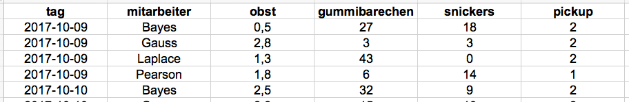
Using df.shape, we can check the structure of the DataFrame, meaning the number of columns and rows. In this case, the dataset contains 15 columns and 891 rows (observations), making it a relatively small dataset. With df.columns, we can display the column names. Now we know what the columns are called, but we still don’t know what the data actually looks like. This can be easily checked using the head or tail function. These functions typically return the first five or last five rows of the dataset. However, using the n parameter, more rows can be displayed. Below, you can see what a DataFrame looks like. For clarity, only the first five columns of the dataset are shown here, but when you run the function yourself, many more columns will be displayed

‍

Anhand dieser ersten Übersicht erkennt man, dass unterschiedliche Skalen in den Daten enthalten sind. Die letzte Funktion, die wir nun vorstellen möchten, um einen ersten Eindruck über Daten zu gewinnen, ist describe. Mit dieser werden typische statistische Metriken wie der Durchschnitt und Median von denjenigen Spalten, die eine metrische Skala besitzen, zurückgegeben. Spalten wie z.B. die Spalte Geschlecht (sex) werden von dieser Funktion nicht berücksichtigt. Das Ergebnis gestaltet sich wie folgt:

‍

Aside from the various metrics for the columns, it is particularly noticeable that in the age column, the number of observations (count) differs from the total number of observations. To investigate this further, we need to take a closer look at the column.

Selecting Data

There are two ways to select columns in Pandas:

# Column selection
# 1. Possibility
df['age']
# 2. Possibility
df.age

‍

The first method always allows you to select a column. The second method is not always guaranteed to work, as column names may contain spaces or special characters. When executing this command, the result is a Series, meaning an n×1 vector. Here, we can see that some observations are missing, indicated by NaN values. How to handle NaN values will be explained at the end of this article. First, we will cover how to select multiple columns or a specific range of a DataFrame.‍‍‍‍

# Selection of several columns
df[['age', 'sex']]
# Selection of a range on an index basis
df.iloc[:2, :3]
# Selection of an area with e.g. column names
df.loc[:3, ['class', 'age']]

‍

Selecting multiple columns is just as straightforward. It is important to ensure that a list of the column names to be selected is created or passed. When selecting a subset of a DataFrame, the iloc or loc functions are used. The former is designed for index-based selection, meaning that instead of passing column names, you specify the position of the column or a range of columns and indices. With the loc function, however, lists and specific column names can be used. In the example above, iloc selects all rows up to index 2 and the first three columns. In contrast, the loc example selects rows up to index 3, along with the age and class columns. These functions provide an entry point for selecting different datasets, but the examples here only scratch the surface of what is possible when it comes to data selection.

Data Manipulation

Finding perfectly structured data in practice would be ideal, but reality often looks quite different. We already encountered an example of this with the age column. To prepare our data for analysis or visualization, we need a way to correct missing values. The fillna function in Pandas provides an effective solution. It automatically selects all NaN values and fills them with predefined replacement values. In our case, we fill the missing age values with the average age. This ensures that no outliers are introduced while keeping the overall average unchanged.

# Filling up NaN values
df.age.fillna(value=df.age.mean())

‍

After calling the functions, we still need to insert the new age column into our dataset; otherwise, the transformation will not be saved. The assignment is very straightforward—by passing the new column name as if selecting an existing column. Afterward, the new values can be accessed easily. Alternatively, we could overwrite the existing age column, but this would mean that the raw data would no longer be visible.

# Assigning new values to a column / creating a new column
df['age_new']=df.age.fillna(value=df.age.mean())

Summary

At the end of this article, we want to briefly summarize some important information about getting started with Pandas:

• Reading data is simple using functions like pd.read_..
• Data is typically structured as a two-dimensional DataFrame
• Functions like df.shape, df.head(), df.tail(), and df.describe() provide an initial overview of the data
• Columns can be selected individually or in multiples by passing their names
• Subsets of a DataFrame are selected using iloc (index-based) or loc (label-based)
• The fillna function allows missing observations to be replaced

As mentioned, this is just an introduction to the Pandas library.

As a preview of our next article in the Data Science with Python series, we will explore the visualization library Matplotlib.