Factor Analysis with Binary Items in SPSS

The assumption of multivariate normally distributed items when conducting an exploratory factor analysis (EFA) strictly speaking prevents the use of binary-scaled items (0/1 coding). While the Pearson correlation coefficient between two binary items corresponds to the phi coefficient, which measures the strength and direction of the relationship between two binary items, the limited value range of a binary item clearly violates the assumption of multivariate normality required for factor analysis.

Using Binary Items in Factor Analysis

To use binary items in an EFA, a so-called polychoric correlation (or in the case of two binary items, the resulting tetrachoric correlation) must be calculated for each item pair. The resulting correlation matrix is then used in the EFA procedure. Polychoric correlations are special correlation coefficients for ordinal data, based on the assumption that each observed item represents an underlying, unobserved (latent) variable, whose continuous value range has been split into ordinal intervals. The method aims to estimate the correlation between these latent variables, rather than relying on their observed ordinal values.

Conducting Factor Analysis with Binary Items

Since SPSS does not currently support polychoric/tetrachoric correlations, the estimation of the correlation matrix must be performed in another software.In a recent project, we implemented the estimation of tetrachoric correlations using the open-source software R and then transferred the resulting correlation matrix to SPSS for conducting the EFA. Below, we briefly outline the key steps of this approach using an exemplary case study.

Step 1: Preparing for Analysis

The R package "foreign" allows the import of SPSS data files (.sav), among other formats. To install it, use the command install.packages("foreign"). Additionally, the R package "polycor" is required to estimate polychoric correlations.

Step 2: Importing Data from SPSS to R

After loading both packages, the SPSS dataset can be imported into R using the function read.spss(). A warning may appear regarding incorrect character encoding or similar issues, but this can usually be ignored.

Step 3: Calculating the Tetrachoric Correlation

To store the calculated correlations, an empty matrix object is created in R. Using a nested loop, the polychoric correlation for each item pair is then computed using the polychor() function. Finally, the diagonal of the correlation matrix must be filled with 1s.

Step 4: Exporting the Correlation Matrix

For further use, the correlation matrix is exported from R as a CSV file using write.table(). It is important to ensure that the correct decimal separator is used (SPSS typically uses a comma, while R uses a period). Below is an example of the R code.

# Install the required packages
install.packages("foreign")
install.packages("polycor")
 
# Load packages
library(foreign)
library(polycor)
 
# Import SPSS data (adjust file path)
data <- read.spss(file="~/Desktop/Binary-Items.sav", 
                  use.value.labels=FALSE, to.data.frame=TRUE)
 
# Number of rows/columns Correlation matrix
n <- ncol(data); m <- n
 
# Create empty correlation matrix
cormat <- matrix(nrow=n, ncol=m, data=NA)
 
# Calculate polychoric correlations for each pair of items
for (i in 1:n){
  for(j in 1:m){
    cormat[i,j] <- polychor(data[,i], data[,j])
  }
}
 
# Set diagonal elements to 1
diag(cormat) <- 1
 
# Export
write.table(cormat, "~/STATWORX/PolyCorMat.csv", row.names=F, sep=";", dec=",")

Step 5: Preparing MATRIX Data in SPSS

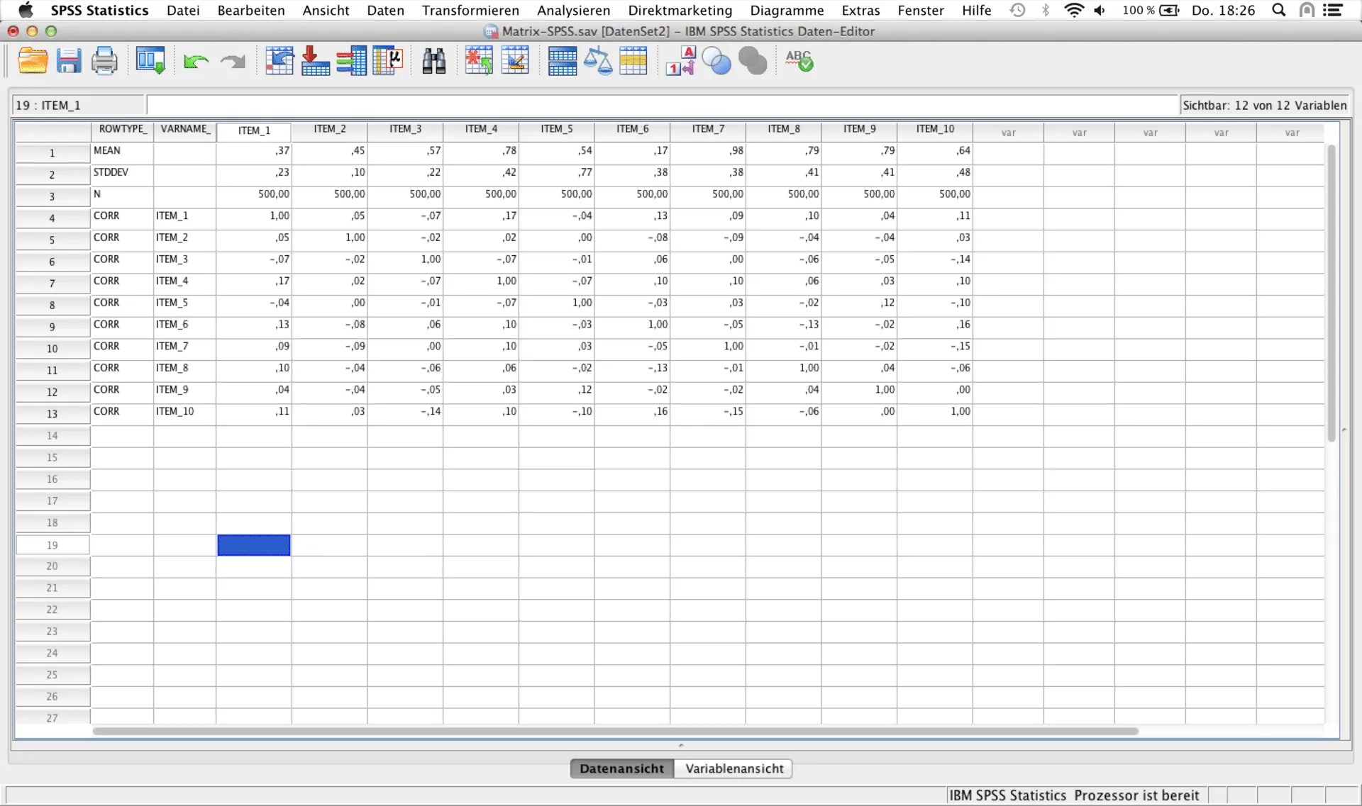
To use the correlation matrix within the FACTOR procedure in SPSS, the matrix must be manually formatted to enable the computation (see screenshot below). The first two columns must contain the attributes ROWTYPE_ and VARNAME_, which need to be created manually by the user. The first three rows must contain the mean (MEAN), standard deviation (STDDEV), and number of observations (N) for each variable. These values can be generated, for example, based on the original dataset in SPSS. The calculated correlations can either be copied and pasted into Excel after import or loaded directly into SPSS.

Step 6: Performing Factor Analysis in SPSS

Once the correlation matrix has been properly formatted, the factor analysis can be conducted. This MUST be done using SPSS syntax, as this is the only way to specify a custom correlation matrix. It is important to ensure that the correlation matrix is the active dataset. The syntax is as follows:

FACTOR MATRIX IN (COR=*)
/MISSING LISTWISE
/PRINT UNIVARIATE INITIAL KMO EXTRACTION ROTATION
/FORMAT BLANK(.30)
/PLOT EIGEN
/CRITERIA MINEIGEN(1) ITERATE(25)
/EXTRACTION PAF
/CRITERIA ITERATE(25)
/ROTATION PROMAX(4)
/METHOD=CORRELATION.

‍

With MATRIX IN (COR=*), SPSS is instructed to use the previously created correlation dataset as the basis for the EFA. In the example above, a principal axis factoring analysis with Promax rotation was performed. Of course, other extraction and rotation methods can also be applied. After running the syntax, the usual results will be displayed in the output window.

Summary

As of now, SPSS does not offer a proper way to incorporate binary items into factor analyses. This is unlikely to change in the future (although SPSS has been implementing more features recently as part of its licensing model restructuring). However, by using open-source software R, these analyses can still be performed within SPSS. Of course, after computing polychoric correlations in R, the entire analysis can also be continued in R. If you have any questions about conducting an exploratory factor analysis with binary items or would like to discuss a specific project, our statistics experts are happy to help at info@statworx.com.

‍