Introduction TensorFlow

TensorFlow is currently one of the most important frameworks for programming neural networks, deep learning models, and other machine learning algorithms. It is based on a C++ low-level backend but is controlled via a Python library. TensorFlow can run on both CPUs and GPUs (including clusters). Recently, an R package has also been introduced, allowing users to utilize TensorFlow within R. TensorFlow is not a software designed for deep learning or data science beginners; rather, it is clearly aimed at experienced users with solid programming skills. However, Keras has been developed as a high-level API that simplifies working with TensorFlow by providing easier functions for implementing standard models quickly and efficiently. This is beneficial not only for deep learning beginners but also for experts who can use Keras to prototype their models more rapidly and efficiently.

The following article will explain the key elements and concepts of TensorFlow and illustrate them with a practical example. The focus will not be on the formal mathematical representation of neural network functionality but rather on the fundamental concepts and terminology of TensorFlow and their implementation in Python.

Tensors

In its original meaning, a tensor described the absolute magnitude of so-called quaternions, complex numbers that extend the range of real numbers. However, this meaning is no longer commonly used today. Today, a tensor is understood as a generalization of scalars, vectors, and matrices. A two-dimensional tensor is essentially a matrix with rows and columns (i.e., two dimensions). In particular, higher-dimensional matrices are often referred to as tensors. However, the concept of a tensor is generally independent of the number of dimensions. Thus, a vector can be described as a one-dimensional tensor. In TensorFlow, tensors flow through what is known as the computation graph.

The Computation Graph

The fundamental functionality of TensorFlow is based on what is known as a computation graph. This refers to an abstract representation of the underlying mathematical problem in the form of a directed graph. The diagram consists of nodes and edges that connect them. The nodes in the graph represent data and mathematical operations in TensorFlow. By correctly connecting the nodes, a computation graph can be created that includes the necessary data and mathematical operations for constructing a neural network. The following example illustrates the basic functionality:

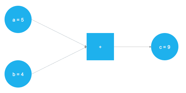
In the above illustration, two numbers are to be added. The two numbers are stored in the variables a and b. The variables flow through the graph until they reach the square box, where an addition is performed. The result of the addition is stored in the variable c. The variables a, b, and c can be understood as placeholders, called "placeholder" in TensorFlow. All numbers assigned to a and b are processed according to the same procedure. This abstract representation of the mathematical operations to be performed is the core of TensorFlow. The following code demonstrates the implementation of this simple example in Python:

# TensorFlow loading
import tensorflow as tf 

# Define a and b as placeholders 
a = tf.placeholder(dtype=tf.int8) 
b = tf.placeholder(dtype=tf.int8) 

# Define the addition 
c = tf.add(a, b) 

# Initialise the graph 
graph = tf.Session() 

# Execute the graph at the point c 
graph.run(c)

First, the TensorFlow library is imported. Then, the two placeholders a and b are defined using tf.placeholder(). Since TensorFlow is based on a C++ backend, the data types of the placeholders must be fixed in advance and cannot be adjusted at runtime. This is done within the function tf.placeholder() using the argument dtype=tf.int8, which corresponds to an 8-bit integer. Using the function tf.add(), the two placeholders are then added together and stored in the variable c. With tf.Session(), the graph is initialized and then executed at c using graph.run(c). Of course, this example represents a trivial operation. The required steps and calculations in neural networks are significantly more complex. However, the fundamental functionality of graph-based execution remains the same.

Placeholders

As previously mentioned, placeholders play a central role in TensorFlow. Placeholders typically contain all the data required for training the neural network. These are usually inputs (the model’s input signals) and outputs (the variables to be predicted).

# Define placeholder 
X = tf.placeholder(dtype=tf.float32, shape=[None, p]) 
Y = tf.placeholder(dtype=tf.float32, shape=[None])

‍

In the above code example, two placeholders are defined. X is intended to serve as a placeholder for the model's inputs, while Y acts as a placeholder for the actual observed outputs in the data. In addition to specifying the data type of the placeholders, the dimension of the tensors stored in them must also be defined. This is controlled via the function argument shape. In the example, the inputs are represented as a tensor of dimension [None, p], while the output is a one-dimensional tensor. The parameter None instructs TensorFlow to keep this dimension flexible, as it is not yet clear at this stage what size the training data will have.

Variables

In addition to placeholders, variables are another core concept of TensorFlow's functionality. While placeholders are used to store input and output data, variables are flexible and can change their values during the computation process. The most important application of variables in neural networks is in the weight matrices of neurons (weights) and bias vectors (biases), which are continuously adjusted to the data during training. The following code block defines the variables for a single-layer feedforward network.

# Number of inputs and outputs 
n_inputs = 10 
n_outputs = 1 

# Number of neurons 
n_neurons = 64 

# Hidden layer: Variables for weights and biases 
w_hidden = tf.Variable(weight_initializer([n_inputs, n_neurons])) 
bias_hidden = tf.Variable(bias_initializer([n_neurons])) 

# Output layer: Variables for weights and biases 
w_out = tf.Variable(weight_initializer([n_neurons, n_outputs])) 
bias_out = tf.Variable(bias_initializer([n_outputs]))

‍

In the example code, n_inputs = 10 inputs and n_outputs = 1 output are defined. The number of neurons in the hidden layer is set to n_neurons = 64. In the next step, the required variables are instantiated. For a simple feedforward network, the weight matrices and bias values between the input and hidden layers are first needed. These are created in the objects w_hidden and bias_hidden using the function tf.Variable(). Within tf.Variable(), the function weight_initializer() is also used, which we will examine in more detail in the next section. After defining the necessary variables between the input and hidden layers, the weights and biases between the hidden and output layers are instantiated.

It is important to understand the dimensions that the required weight and bias matrices must take to be processed correctly. A general rule of thumb for weight matrices in simple feedforward networks is that the second dimension of the previous layer represents the first dimension of the current layer. While this may initially sound complex, it essentially refers to the passing of outputs from layer to layer in the network. The dimension of the bias values typically corresponds to the number of neurons in the current layer. In the above example, the number of inputs and neurons results in a weight matrix of the form [n_inputs, n_neurons] = [10, 64], as well as a bias vector in the hidden layer with a size of [bias_hidden] = [64]. Between the hidden and output layers, the weight matrix has the form [n_neurons, n_outputs] = [64, 1], while the bias vector has the form [1].

Initialization

In the code block from the previous section, the functions weight_initializer() and bias_initializer() were used when defining the variables. The way in which the initial weight matrices and bias vectors are filled has a significant impact on how quickly and effectively the model can adapt to the given data. This is because neural networks and deep learning models are trained using numerical optimization methods, which always begin adjusting the model’s parameters from a specific starting position. Choosing an advantageous starting position for training the neural network generally has a positive effect on computation time and the model’s fit.

TensorFlow provides various initialization strategies, ranging from simple matrices with constant values, such as tf.zeros_initializer(), to random values, such as tf.random_normal_initializer() or tf.truncated_normal_initializer(), and even more complex functions like tf.glorot_normal_initializer() or tf.variance_scaling_initializer(). Depending on the initialization of the weights and bias values, the outcome of model training can vary significantly.‍

# Initializers 
weight_initializer = tf.variance_scaling_initializer(mode="fan_avg", distribution="uniform", scale=1) 
bias_initializer = tf.zeros_initializer()

‍

In our example, we use two different initialization strategies for the weights and bias values. While tf.variance_scaling_initializer() is used for initializing the weights, we use tf.zeros_initializer() for the bias values.

Network Architecture Design

After implementing the necessary weight and bias variables, the next step is to create the network architecture, also known as topology. In this step, placeholders and variables are combined using successive matrix multiplications.

Additionally, when specifying the topology, the activation functions of the neurons are defined. Activation functions apply a nonlinear transformation to the outputs of the hidden layers before passing them to the next layer. This makes the entire system nonlinear, allowing it to adapt to both linear and nonlinear functions. Over time, numerous activation functions for neural networks have been developed. The current standard in deep learning model development is the so-called Rectified Linear Unit (ReLU), which has proven to be advantageous in many applications.

# Hidden layer 
hidden = tf.nn.relu(tf.add(tf.matmul(X, w_hidden), bias_hidden)) 

# Output layer 
out = tf.transpose(tf.add(tf.matmul(hidden, w_out), bias_out))

‍

ReLU activation functions are implemented in TensorFlow using tf.nn.relu(). The activation function takes the output of the matrix multiplication between the placeholder and the weight matrix, along with the addition of the bias values, and transforms them: tf.nn.relu(tf.add(tf.matmul(X, w_hidden), bias_hidden)). The result of this nonlinear transformation is passed as output to the next layer, which then uses it as input for another matrix multiplication. Since the second layer in this example is already the output layer, no additional ReLU transformation is applied. To ensure that the dimensionality of the output layer matches that of the data, the matrix must be transposed using tf.transpose(). Otherwise, issues may arise when estimating the model.

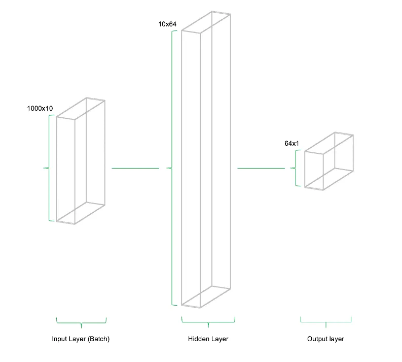
The above illustration schematically depicts the architecture of the network. The model consists of three parts: (1) the input layer, (2) the hidden layer, and (3) the output layer. This architecture is called a feedforward network. "Feedforward" describes the fact that data flows through the network in only one direction. Other types of neural networks and deep learning models include architectures that allow data to move "backward" or in loops within the network.

Cost Function

The cost function of the neural network is used to compute a measure of the deviation between the model’s prediction and the actually observed data. Depending on whether the problem is classification or regression, different cost functions are available. For classification tasks, cross-entropy is commonly used, while for regression problems, the mean squared error (MSE) is preferred. In principle, any mathematically differentiable function can be used as a cost function.

# Cost function 
mse = tf.reduce_mean(tf.squared_difference(out, Y))

‍

In the above example, the mean squared error is implemented as the cost function. TensorFlow provides the functions tf.reduce_mean() and tf.squared_difference(), which can be easily combined. As seen in the code, the function arguments for tf.squared_difference() include the placeholder Y, which contains the actually observed outputs, and the object out, which holds the model-generated predictions. The cost function thus brings together the observed data and the model’s predictions for comparison.

Optimizer

The optimizer is responsible for adjusting the network’s weights and bias values during training based on the computed deviations from the cost function. To achieve this, TensorFlow calculates the so-called gradients of the cost function, which indicate the direction in which the weights and biases need to be adjusted to minimize the model’s cost function. The development of fast and stable optimizers is a major research field in neural networks and deep learning.

# Optimizer 
opt = tf.train.AdamOptimizer().minimize(mse)

‍

In this case, the tf.AdamOptimizer() is used, which is currently one of the most commonly applied optimizers. Adam stands for Adaptive Moment Estimation and is a methodological combination of two other optimization techniques (AdaGrad and RMSProp). At this point, we do not delve into the mathematical details of the optimizer, as this would go beyond the scope of this introduction. The key takeaway is that different optimizers exist, each based on distinct strategies for computing the necessary adjustments to weights and biases.

Session

The TensorFlow session serves as the fundamental framework for executing the computational graph. The session is initiated using the command tf.Session(). Without starting the session, no computations within the graph can be performed.

# Start session 
graph = tf.Session()

‍

In the code example, a TensorFlow session is instantiated in the object graph and can subsequently be executed at any point within the computational graph. In the latest development versions (Dev-Builds) of TensorFlow, there are emerging approaches to executing code without explicitly defining a session. However, this feature is not yet included in the stable build.

Training

Once the necessary components of the neural network have been defined, they can now be linked together during the model training process. The training of neural networks today is typically conducted using a method called "minibatch training." Minibatch means that random subsets of inputs and outputs are repeatedly selected to update the network's weights and biases. To facilitate this, a parameter is defined to control the batch size of the randomly sampled data. Generally, data is drawn without replacement, meaning that each observation in the dataset is presented to the network only once per training round (also called an epoch). The number of epochs is also defined by the user as a parameter.

The individual batches are fed into the TensorFlow graph using the previously created placeholders X and Y through a feed dictionary. This process is executed in combination with the previously defined session.

# Transfer current batch to network 
graph.run(opt, feed_dict={X: data_x, Y: data_y})

‍

In the above example, the optimization step opt is performed within the graph. For TensorFlow to execute the necessary computations, data must be passed into the graph using the feed_dict argument, replacing the placeholders X and Y.

Once the data is passed via feed_dict, X is fed into the network through multiplication with the weight matrix between the input and hidden layers and is then nonlinearly transformed by the activation function. The hidden layer's output is subsequently multiplied by the weight matrix between the hidden and output layers and passed to the output layer. At this stage, the cost function calculates the difference between the network’s prediction and the actual observed values Y. Based on the optimizer, gradients are computed for each individual weight parameter in the network. These gradients determine how the weights are adjusted to minimize the cost function. This process is known as gradient descent. The described procedure is then repeated for the next batch. With each iteration, the neural network moves closer to minimizing the cost, reducing the deviation between predictions and observed values.

Application Example

In the following example, the previously discussed concepts will be demonstrated using a practical application. To proceed, we first need some data on which the model can be trained. These can be easily and quickly simulated using the function sklearn.datasets.make_regression() from the sklearn library.

# Number of inputs, neurons and outputs 
n_inputs = 10 
n_neurons = 64 
n_outputs = 1 

# Simulate data for the model 
from sklearn.datasets import make_regression 
data_x, data_y = make_regression(n_samples=1000, n_features=n_inputs, n_targets=n_outputs)

‍

As in the above example, we use 10 inputs and 1 output to create a neural network for predicting the observed output. We then define placeholders, initialization, variables, network architecture, cost function, optimizer, and session in TensorFlow.

# Define placeholder 
X = tf.placeholder(dtype=tf.float32, shape=[None, n_inputs]) 
Y = tf.placeholder(dtype=tf.float32, shape=[None]) 

# Initializers 
weight_initializer = tf.variance_scaling_initializer(mode="fan_avg", distribution="uniform", scale=1) 
bias_initializer = tf.zeros_initializer() 

# Hidden layer: Variables for weights and biases 
w_hidden = tf.Variable(weight_initializer([n_inputs, n_neurons])) 
bias_hidden = tf.Variable(bias_initializer([n_neurons])) 

# Output layer: Variables for weights and biases 
w_out = tf.Variable(weight_initializer([n_neurons, n_outputs])) 
bias_out = tf.Variable(bias_initializer([n_outputs])) 

# Hidden Layer 
hidden = tf.nn.relu(tf.add(tf.matmul(X, w_hidden), bias_hidden)) 

# Output Layer 
out = tf.transpose(tf.add(tf.matmul(hidden, w_out), bias_out)) 

# Cost function 
mse = tf.reduce_mean(tf.squared_difference(out, Y)) 

# Optimizer 
opt = tf.train.AdamOptimizer().minimize(mse) 

# Start session 
graph = tf.Session()

‍

Now, the model training begins. For this, we first need an outer loop that runs through the number of defined epochs. Within each iteration of the outer loop, the data is randomly divided into batches and sequentially fed into the network through an inner loop. At the end of each epoch, the MSE (mean squared error) of the model compared to the actual observed data is calculated and displayed.

# Batch size 
batch_size = 256 

# Number of possible batches 
max_batch = len(data_y) // batch_size 

# Number of epochs 
n_epochs = 100 

# Training of the model 
for e in range(n_epochs): 
    # Random arrangement of X and Y for minibatch training 
    shuffle_indices = np.random.randint(low=0, high=n, size=n) 
    data_x = data_x[shuffle_indices] 
    data_y = data_y[shuffle_indices] 
 
    # Minibatch training 
    for i in range(0, max_batch): 
       # Batches erzeugen 
        start = i * batch_size 
        end = start + batch_size 
        batch_x = data_x[start:end] 
        batch_y = data_y[start:end] 

        # Transfer current batch to network 
        net.run(opt, feed_dict={X: batch_x, Y: batch_y}) 

    # Display the MSE per epoch 
    mse_train = graph.run(mse, feed_dict={X: data_x, Y: data_y}) 
    print('MSE: ' + str(mse))

‍

A total of 15 batches are presented to the network per epoch. Within 100 epochs, the model is able to reduce the MSE from an initial 20,988.60 to 55.13 (Note: These values vary from run to run due to the random initialization of weights and biases as well as the random selection of batches). The figure below shows the progression of the mean squared error during training.

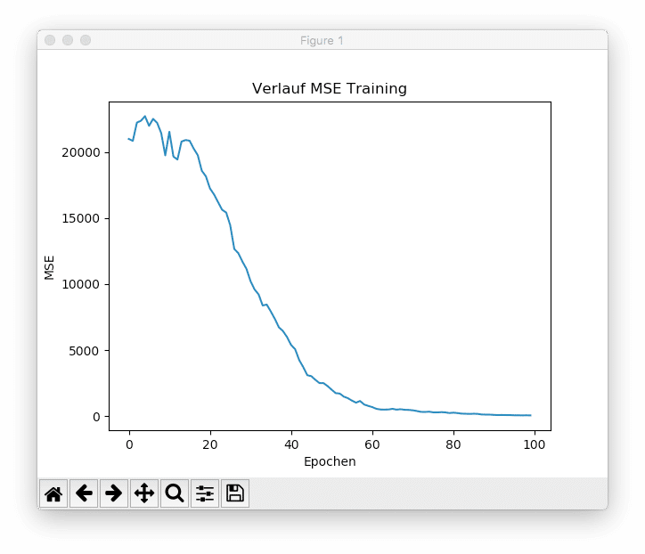
It can be seen that with a sufficiently high number of epochs, the model is able to reduce the training error to nearly zero. While this might initially seem beneficial, it poses a problem for real-world machine learning projects. Neural networks often have such high capacity that they simply "memorize" the training data and fail to generalize well to new, unseen data. This phenomenon is called overfitting the training data. For this reason, the prediction error on unseen test data is often monitored during training. Typically, model training is stopped at the point where the test data’s prediction error begins to increase again. This technique is known as early stopping.

Summary and Outlook

With TensorFlow, Google has set a milestone in deep learning research. Thanks to Google's vast intellectual capacity, they have created software that has quickly established itself as the de facto standard for developing neural networks and deep learning models. At statworx, we also successfully use TensorFlow in our data science consulting services to develop deep learning models and neural networks for our clients.