Introduction to Methods: The t-Test

One of the most commonly used statistical tests is the t-test. It can be used, among other things, to check whether the mean of a random variable corresponds to a specific value. It can also be used to compare two means. As with any other statistical test, certain prerequisites must be met for the t-test to be used reliably:

• Normal distribution of the random variables
• Independence of observations
• Homogeneity of variance (in the two-group case)

If these prerequisites are not met, all is not lost! The robustness of the t-test allows the normal distribution to become less important with larger sample sizes(1). For small samples, there are non-parametric alternatives, such as the Wilcoxon rank-sum test. A description of this test can be found here.

Formulas for Different Cases

Where exactly does independence play a role? It is important to distinguish between different cases for this. If you have only one variable, the independence refers to the individual observations among themselves. When comparing two random variables, the following cases may occur, leading to different calculations of the test statistic:

‍

Hierbei stehen

• $sigma$ for variance
• $S$ for the estimated variances
• $S = frac{ (n_{x}-1) cdot S_{x}^{2}+ (n_{y}-1) cdot S_{y}^{2} }{ n_{x} + n_{y} -2 }$
• $S_{D}^{2} = frac{ 1 }{ n-1 } sum_{ i = 1 }^n (D_{i}-bar{D})$

To check the prerequisites, the substantive aspect of the variables should be used alongside other statistical tests. The question of whether it is a paired sample can already be clarified by examining the investigation methodology. For example, if a group was examined before and after a treatment, it is a paired (also called connected) sample.

Once the prerequisites have been checked and the t-test conducted, the actual interpretation of the results begins. What exactly do the numbers mean? What conclusions can be drawn? Is the result significant? These questions are to be clarified with a small example.

Example for SPSS Outputs

We simulated a total of 400 observations - let's say it's the sleep duration in hours. We assume the following three scenarios:

1. all data come from one group (test with a single sample)
2. the data come from one group in a before-and-after comparison (test with paired samples)
3. the data come from two different groups (test with independent samples)

In SPSS, there are exactly these three cases for the t-test: with a single sample, with independent samples, and with paired samples. The output differs slightly, as can be seen in the illustrations. Nevertheless, the essential interpretations are the same.

‍

‍

‍

The following values are always given:

• the value of the test statistic "T"
• the number of degrees of freedom "df" (degree of freedom)
• the p-value "Sig. (2-sided)"
• the "Lower" and "Upper" limit of the confidence interval
• the "Mean" or "Mean Difference"

These key figures are strongly interconnected. The p-value is determined using the value of the test statistic and the degree of freedom. The limits of the confidence interval are another representation of whether a test is significant or not. They have the same significance as the p-value. The "Mean" or "Mean Difference" indicates the deviation of the data either to the mean or among the groups. It helps put the statement of the t-test in relation to the question: Which group is larger? In which direction does the effect point?

The output of the t-test with independent samples also contains the Levene test. This is used to check the equality of variance ($H_{0}: sigma_{1} = sigma_{2}$). Depending on whether there is significance here, the corresponding row of the table must be used for evaluation. The values of the two rows may differ, which is attributable to the previously mentioned, different formulas.

Evaluation

What does this mean for our example? As can be seen, the key figures in the three tests are different.

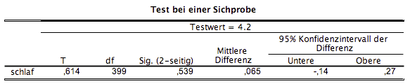
Scenario - Test with a Single Sample
There is no significant indication here that the mean is not 4.2 in the entire data.

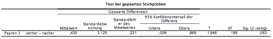
Scenario - Test with Paired Samples
The difference between before and after is just barely not significant for $alpha = 0,05$

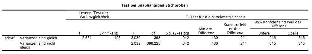
Scenario - Test with Independent Samples
It shows that variance homogeneity can be assumed, and there is a significant difference in the groups for $alpha = 0,05$

Summary

The different t-tests can deliver different results due to differences in calculation. This can even affect significance in extreme cases - as in our example. Therefore, it is important to be clear in advance about the structure of the data you are examining.

References

1. Eid, Gollwitzer, Schmitt (2015) Statistics and Research Methods, Chapter: 12.1, p. 369ff

‍