Data Science in Python - Getting started with Machine Learning with Scikit-Learn

In our previous articles on Data Science in Python, we have covered basic syntax, data structures, arrays, data visualization, and manipulation/selection. What is still missing for a proper introduction is the ability to apply models to the data in order to recognize patterns and derive predictions. The variety of implemented models in Python, especially in Scikit-Learn, allows for a great deal of flexibility in customizing models.
Machine Learning Libraries for Python
The most well-known ML library that has evolved significantly in recent years is TensorFlow by Google. It is primarily used for developing and training neural networks. Other well-known libraries include Keras, PyTorch, Caffe, and MXNet. More information on how neural networks work can be found in another blog post of ours. However, it is important to keep in mind that neural networks are just one subfield of machine learning. Decision trees, random forests, and support vector machines are also considered ML models. For beginners in this field, it is therefore advisable to choose a library that covers all these models rather than focusing solely on a single subfield like neural networks. Scikit-Learn is one such library. Its consistent syntax greatly simplifies both model development and the application of data to models.
Getting Started with Scikit-Learn
The first release of Scikit-Learn took place in 2010, and it has been continuously developed ever since. Today, the codebase includes more than 150,000 lines of code. Installation, like with other libraries, is done using pip or conda:
pip install scikit-learn
conda install scikit-learn
Scikit-Learn divides its various sublibraries based on the specific machine learning task:
- Classification (Example: Does the customer belong to category A, B, or C?)
- Regression (Example: What sales volume can be expected next month?)
- Clustering (Example: How can customers be segmented into different groups?)
- Dimensionality Reduction
- Model Selection
- Preprocessing
The sublibraries can be imported as follows: import sklearn.cluster as cl. For the Classification and Regression sublibraries, this applies only to a limited extent, as ML models can be used for both regression and clustering. However, the functionality remains similar.
# Neuronales Netz zur Klassifikation
from sklearn.neural_network import MLPClassifier
# Neuronales Netz zur Regression
from sklearn.neural_network import MLPRegressor
Structure of Model Training
Depending on the ML problem being addressed, the categorization above provides a quick overview of the available models in Scikit-Learn. The process of model training is always the same:
# Import des Entscheidungsbaum
from sklearn import tree

# Beispieldaten
X = [[0, 0], [1, 1]]
Y = [0, 1]

# Initialisierung des Entscheidungsbaum zur Klassifizierung
clf = tree.DecisionTreeClassifier()

# Training des Entscheidungsbaums
clf = clf.fit(X, Y)

# Prädiktion für neue Daten
clf.predict([[2., 2.]])
The first step is to initialize the model, where model parameters can be specified in more detail. These parameters are always documented, such as in this example. If no parameters are provided, Scikit-Learn uses the model’s default configuration. This can be very useful for an initial test to determine whether a model can even be applied to the data. However, it should not immediately be considered a disqualifying factor if the model performance does not meet expectations. In the next step, the model is trained using the fit method, and new data can be fed into the model using the predict method.
Now, we want to expand on the previous minimal example and work with actual data. The goal of training the decision tree is to determine, based on the features age, gender, and booking class, whether a passenger survived the Titanic disaster. We previously used the Titanic dataset in our blog post on Pandas.
After importing the data, we first need to transform the gender variable, as the decision tree cannot be trained with string-format data. Next, we extract the relevant training columns and simultaneously remove missing data entries. The most important step is then splitting the data into training and test sets, as model performance must be evaluated using data that was not used for training. A 70% training / 30% test split is a good general rule of thumb. The decision tree is then trained, with its depth limited to five in this case. Finally, the accuracy for the test data is calculated.
import seaborn as sns
from sklearn import preprocessing
from sklearn.model_selection import train_test_split
from sklearn.tree import DecisionTreeClassifier

# Laden der Daten
df = sns.load_dataset('titanic')

# Transformation der Variable Geschlecht
labelenc = preprocessing.LabelEncoder()
labelenc.fit(df.sex)
df['sex_transform'] = labelenc.transform(df.sex)

# Auswahl von Daten zum Training
train = df.loc[:,['age', 'fare', 'sex_transform', 'survived']].dropna()

# Aufteilen der Daten in Features und Target
y = train['survived']
X = train.drop('survived', axis=1)

# Aufteilen in Test und Train Daten
X_train, X_test, y_train
y_test = train_test_split(X, y, test_size=0.4, random_state=10, shuffle = True)

# Initialisierung des Entscheidungsbaums
clf = DecisionTreeClassifier(max_depth=5)

# Training des Entscheidungsbaums
clf.fit(X_train, y_train)

# Berechnung der Metrik
clf.score(X_test, y_test)
This process is very similar for other models since Scikit-Learn implements nearly the same methods for every model. For example, a Random Forest model would follow this structure:
from sklearn.ensemble import RandomForestClassifier

# Initialisierung des Random Forest Modells
rf = RandomForestClassifier()

# Training des Random Forest Modells
rf.fit(X_train, y_train)

# Berechnung der Metrik
rf.score(X_test, y_test)
This syntax runs like a common thread throughout the Scikit-Learn library.
Tuning the Model’s Hyperparameters
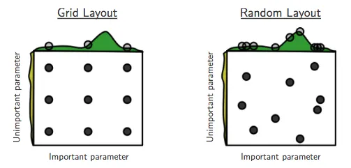
One challenge in applying machine learning models is determining the optimal model parameters. The number of variations is so vast that manually testing each combination is impractical. For this process, the so-called GridSearch method can be used. It creates a grid of all possible parameter combinations—the more parameters and variations are tested, the larger the grid becomes. If there are too many combinations, selecting random parameter combinations can be useful, as this speeds up the process and makes it easier to find suitable parameter settings. The following graphic further illustrates this comparison:
Now, we introduce the full Grid-Search method:
from sklearn.model_selection import GridSearchCV

# Definition der Paramerkombination
params = {"max_depth": range(3,15), "splitter": ["best", "random"]}

# Erstellen des Grids
grid = GridSearchCV(estimator=clf, param_grid=params,
                    cv=10, verbose=2, n_jobs=-1)

# Training des Grids
grid.fit(X_train, y_train)
print(grid.best_params_, grid.best_score_)
The parameter combinations to be evaluated are defined in a dictionary, where each key corresponds to a model parameter. Each key is assigned a list of different options, in this case, the depth of the decision tree and the splitting method. The grid object must be initialized similarly to the model. By using the n_jobs parameter, optimization is performed in parallel, making the process faster. Finally, the best parameter combination and its corresponding score can be displayed. It is essential to evaluate the model using test data afterward. There is no universal answer as to which parameters are suitable for which model type, as this often depends on the characteristics of the data.
Recap
In this blog post, we explained the functionality of machine learning models using a decision tree with Scikit-Learn. The key steps are always to initialize the model, then train it (fit), generate predictions (predict), and evaluate accuracy (score). Scikit-Learn enables the implementation of many other model types and applications. For example, the entire data preprocessing and training process can be combined into pipelines. My colleague Martin has summarized how to do this in his article.
This post marks the conclusion of our introduction to Python for Data Science.
References
- Bergstra, Bengio (2012): Random Search for Hyper-Parameter Optimization


