Deep Learning - Part 2: Programming

Building on the theoretical introduction to neural networks and deep learning from the last blog post, Part 2 of the "Deep Learning" series will provide a hands-on demonstration of implementing a simple neural network (feedforward network) in Python. Various frameworks are available to users for this purpose. In this post, we will use Keras, one of the most important Python libraries for programming neural networks and deep learning models.

Overview of Deep Learning Frameworks

In recent years, the deep learning software ecosystem has seen many new additions. Numerous frameworks offering predefined building blocks for constructing deep learning networks have been introduced to the open-source community. These include Torch, used by Facebook, whose high-level interface utilizes the scripting language Lua; Caffe, which enjoys great popularity in academic settings; Deeplearning4j, which provides a Java-based deep learning environment; and Theano, which focuses on mathematically efficient computations. In addition to the aforementioned frameworks, many other libraries allow users to program both simple and complex deep learning models. These notably include Apache MxNet and Intel Nervana NEON. However, the largest and most resource-rich deep learning framework currently is TensorFlow, originally developed by the Google Brain Team and now released as open-source software. TensorFlow is implemented in C++ and Python but can also be integrated and used in other languages such as R, Julia, or Go, with varying degrees of effort. Most recently, Python has become the lingua franca of deep learning model programming, primarily due to TensorFlow and its high-level library, Keras.

Google TensorFlow

TensorFlow is a software library for Python that allows mathematical operations to be modeled as a graph. This graph serves as a framework in which data is mathematically transformed at each node and then passed on to subsequent nodes. The data is stored and processed in so-called tensors. A tensor, simply put, is a container that holds the values computed within the graph. The following illustration and the Python code snippet below aim to illustrate this with a simple example:

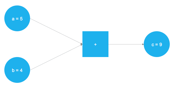
The graph defines a simple mathematical operation—an addition in this case. The values (tensors) a and b are added at the square node of the graph, forming the value c. In TensorFlow, this looks as follows:

# TensorFlow laden
import tensorflow as tf
# a und b als Konstanten definieren
a = tf.constant(5)
b = tf.constant(4)
# Die Addition definieren
c = tf.add(a, b)
# Den Graphen initialisieren
graph = tf.Session()
# Den Graphen an der Stelle c ausführen
graph.run(c)

‍

The result of the computation is 9. This simple example quickly reveals the fundamental logic behind TensorFlow. In the first step, an abstract concept of the model to be computed is created (the graph), which is then populated with tensors in the next step and executed and evaluated at a specific point. Of course, graphs for deep learning models are significantly more complex than the minimal example above. TensorFlow provides users with the TensorBoard function, which allows the programmed graph to be visualized in great detail. An example of a more complex graph can be seen in the figure below.

Since TensorFlow allows the definition of arbitrary mathematical operations, it is not strictly a pure deep learning framework. Other machine learning models can also be represented as graphs and computed using TensorFlow. However, TensorFlow was primarily developed with a focus on deep learning and comes with numerous predefined building blocks for implementing neural networks (e.g., prebuilt layers for MLPs or CNNs). After the release of version 1.0 in 2016 and significant progress in the TensorFlow API, a certain level of stability and code consistency can be expected in the coming years. This will further support the widespread adoption of TensorFlow and its use in production systems. In addition to the Python library, there is also a TensorFlow server designed for enterprise use, which provides ready-made TensorFlow models as a service.

Introduction to Keras

Despite the prebuilt blocks mentioned earlier, TensorFlow is still an expert system and requires a significant learning curve for users. The relative development time from the initial idea to a fully functional deep learning model is extremely long in TensorFlow—but it is also highly flexible.

Keras aims to mitigate the lengthy exploration time common in most deep learning frameworks by providing an easy-to-use interface for building deep learning models. By using a simpler syntax, Keras streamlines the design, training, and evaluation of deep learning models. Fundamentally, Keras operates at the abstraction level of individual neural network layers and typically connects them automatically. This eliminates most concerns regarding network architecture details or their implementation. As a result, standard models such as MLPs, CNNs, and RNNs can be quickly and efficiently prototyped. What makes Keras unique is that it does not provide its own computation backend; instead, it simplifies access to underlying libraries such as TensorFlow, Theano, or CNTK. One advantage of this approach is that the code specifying network architectures remains the same across all backends and is automatically "translated" by Keras. This enables extremely fast development in different frameworks without requiring deep familiarity with their complex syntax. Consequently, Keras code is significantly shorter and more readable compared to its equivalent in the native syntax of the respective backend framework.

Example: Implementing a Neural Network

The following code examples use the Python API of Keras to implement deep learning models. The example focuses on predicting the S&P 500 price for the next trading minute based on the prices of the individual stocks in the index. This example is solely intended to demonstrate the implementation of a neural network and is not optimized for performance. (It is worth noting here that forecasting stock and index prices remains extremely challenging, particularly as time intervals become shorter. An interesting approach to ensemble-based stock prediction is taken by the AI fund NUMERAI.)

The dataset for model training consists of minute-by-minute trading prices of the underlying stocks and the index itself from April to July 2017. Each row of the training dataset contains the prices of all index components as features for the prediction, along with the index price for the next minute as the target. The test dataset consists of the same type of data for August 2017.

The following section explains the Python model specification in Keras, assuming that the DataFrames containing the training and test data are already available:

# Layer aus der Keras Bibliothek laden
from keras.layers import Dense
from keras.models import Sequential

‍‍

First, the necessary components are imported from Keras. These include the classes for a fully connected layer (Dense), the model type (Sequential), and the main library for computations.

# Initialisierung eines leeren Netzes
model = Sequential()
# Hinzufügen von 2 Feedforward Layern
model.add(Dense(512, activation="relu", input_shape=(ncols,)))
model.add(Dense(256, activation="relu"))
# Output Layer
model.add(Dense(1))

‍‍

Next, the framework of the model is defined within an object (model). After instantiating the container for the model, two hidden layers with 512 and 256 neurons, respectively, and the ReLU activation function are added. The final layer of the model, the output layer, sums up the previously computed outputs of the preceding nodes and weights them accordingly.

# Modell kompilieren
model.compile(optimizer="adam", loss="mean_squared_error")
# Modell trainieren mit den Trainingsdaten
model.fit(x=stockdata_train_scaled,
          y=stockdata_train_target,
          epochs=100, batch_size=128)
# Geschätztes Modell auf den Testdaten evaluieren
results = model.evaluate(x=stockdata_test_scaled, y=stockdata_test_target)

‍‍

After defining the network architecture, the model is compiled along with the training parameters. Since this is a regression problem, the Mean Squared Error (MSE) is used as the loss function. The MSE calculates the average squared deviation between the actual observed values and the values predicted by the network in each iteration. During training, the MSE is iteratively minimized using an adaptive gradient method (ADAM). Through backpropagation, the weights between neurons are adjusted so that the MSE decreases (or at least should) with each iteration. In this example, 100 epochs were chosen as the training duration, but in a real-world application, this parameter should also be optimized through extensive testing. One epoch corresponds to a complete pass through the data, meaning that the network has "seen" every data point in the training set once.

Results and Outlook

As shown in the following figure, the result is not ideal. The blue line represents the actual S&P 500 index values, while the model’s prediction is shown in orange.

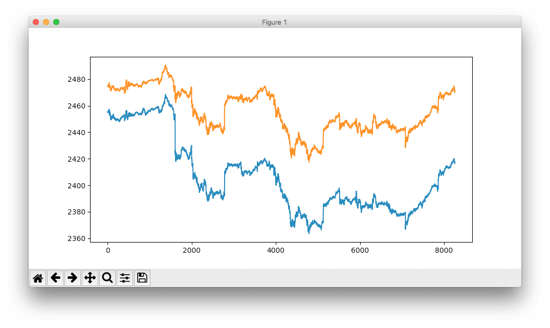
Interestingly, even the non-optimized network has already learned the overall structure of the trend, although it significantly overestimates fluctuations and effects.

In the next post in the "Deep Learning" series, we will build on this work and further improve our model’s performance by applying various tuning approaches.