How deep does MLP Deep Learning need to be?


As already mentioned in the first part of our introduction series on deep learning, neural networks and deep learning are currently an active area of machine learning research. While the underlying ideas and concepts have been around for several decades, the complexity of models and architectures has steadily increased in recent years. In this blog post, we explore whether adding more hidden layers in the context of feedforward networks necessarily improves model quality or whether the increased complexity of the model is not always beneficial. The practical example of S&P 500 forecasting corresponds to the setting already known from part 2 of the introduction series.
Deep Learning – The Importance of the Number of Layers and Neurons
he team led by Geoffrey Hinton first demonstrated in 2006 that training a multilayer neural network is possible. Since then, the so-called depth of a neural network, i.e., the number of layers used, has become a potential hyperparameter of the model. This means that during the development of the neural network, the predictive quality of the model should also be tested across networks of varying depths. From a theoretical perspective, increasing the number of layers leads to better or more complex abstraction capabilities of the model, as the number of computed interactions between inputs increases. However, strictly increasing the number of neuron layers can also lead to problems. On the one hand, deep network architectures risk rapid overfitting to training data. This means that due to its increased capacity, the model quickly learns specific properties of the training data that have no relevance for generalizing to future test data. Furthermore, increased model complexity also leads to a more complex scenario in terms of parameter estimation for the model. All neural networks and deep learning models are trained using numerical optimization methods. New neuron layers require additional parameters to be estimated, making the optimization problem more challenging. As a result, in very complex model architectures, it may not be possible to find a sufficiently good solution to the underlying optimization problem. This, in turn, negatively affects the quality of the model. The number of layers in a neural network is just one of many hyperparameters that must be considered when designing the model architecture. Besides the number of layers, another important aspect is the number of neurons per layer. Despite intensive efforts and research in this area, it has not yet been possible to establish a universally valid concept regarding the architecture of neural networks. Jeff Heaton, a well-known author of several introductory works on deep learning, provides the following general rules of thumb in his books(1):
- The number of neurons should be between the size of the input and output layer.
- The number of neurons in the first layer should be about 2/3 of the size of the input layer.
- The number of neurons should not exceed twice the size of the input layer.
These recommendations are helpful for deep learning beginners but hardly claim universal validity. The architecture of the network usually needs to be redesigned from problem to problem.
Empirical Example
The figure below shows the predictions of two neural networks (orange, blue) as well as the original values (gray). The blue model has a single neuron layer, while the orange model has four layers. Both models were trained for 10 epochs. It is easy to see that adding more layers leads to an observed improvement in model quality.
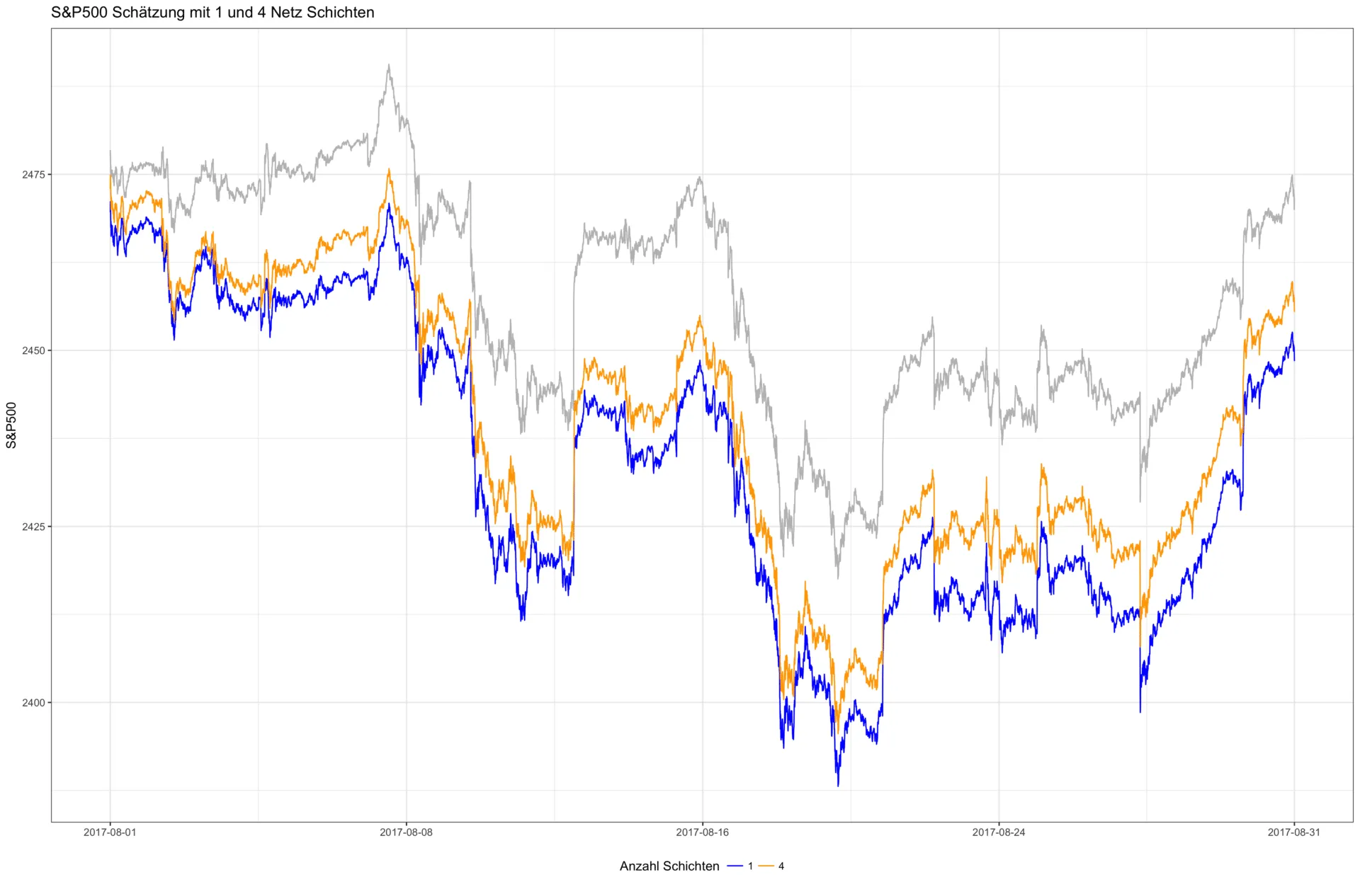
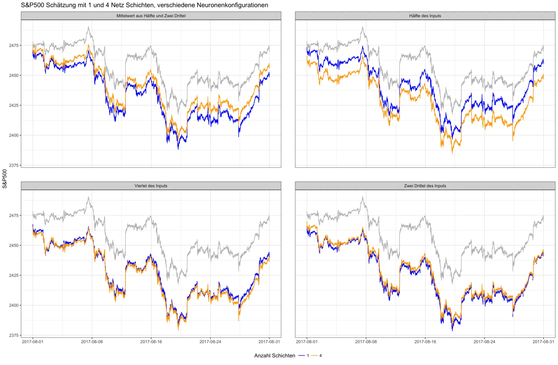
However, this example should not lead to the conclusion that adding more layers always results in an improvement. In addition to the already mentioned overfitting problem, it is often simply unnecessary to design a deep network for simple problems. For example, it can be mathematically proven that a neural network with just one layer and a finite number of neurons can approximate any continuous function—under mild assumptions regarding the activation function of the neurons. This is known as the universal approximation theorem. In the second experiment, we examine the interplay between network depth and the number of neurons. In the figure below, various neuron configurations of individual layers were trained alongside a varying network depth. The number of neurons in the first layer always depends on the size of the input layer—that is, the number of input features used. For example, the configuration "half of the inputs" for the 500 input factors used here (all S&P 500 stocks) results in the following number of neurons per layer: 250, 125, 63, 32, 16. In this experiment, each subsequent layer halves the number of neurons in the previous layer to increasingly condense the extracted information.
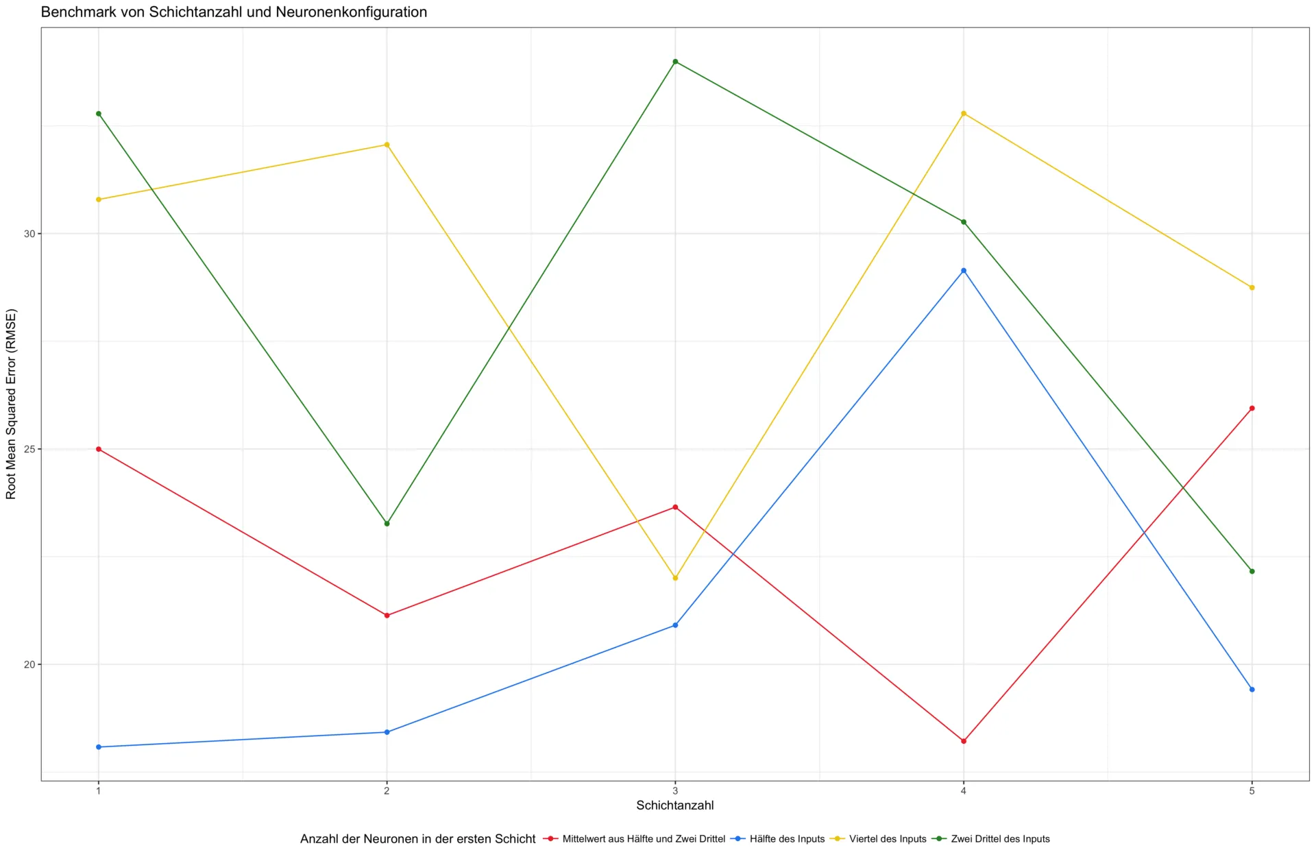
The effect of a deeper network is therefore not always positive. This becomes particularly evident in the next graph. Here, the average prediction error is plotted as a function of the same neuron configurations and varying network depths—from one to five layers. No generally lower error can be observed for deeper networks.
Result and Outlook
How can the results of this experiment be summarized? The most important point is that there is no "standard recipe" even for simple neural networks. In the machine learning context, this is also known as the "no free lunch theorem." Furthermore, it can be stated that more layers are not necessarily better. Even for simple architectures, the number of layers and the neuron configuration should be treated as variable hyperparameters and optimized for the given task using cross-validation. There are various approaches for this, such as incrementally building a network until a target performance is achieved or pruning large networks by gradually removing unimportant neurons (those that are never activated). The rules of thumb from Heaton and others can serve as good starting points but do not replace extensive model tuning.
References
- Heaton, Jeff (2008): Introduction to Neural Networks for Java


